Polar coordinates

The biharmonic equation in polar coordinates is written explicitly as:

\[\newcommand{\vx}{r} \newcommand{\vy}{\theta} \newcommand{\lx}{L_{\vx}} \newcommand{\ly}{L_{\vy}} \newcommand{\ux}{u_{\vx}} \newcommand{\uy}{u_{\vy}} \frac{1}{\vx} \pder{}{}{\vx} \left( \vx \pder{}{}{\vx} \left( \frac{1}{\vx} \pder{}{}{\vx} \left( \vx \pder{}{\psi}{\vx} \right) \right) \right) + 2 \frac{1}{\vx} \pder{}{}{\vy} \left( \frac{1}{\vx} \pder{}{}{\vy} \left( \pder{}{}{\vx} \pder{}{\psi}{\vx} \right) \right) + \frac{1}{\vx} \pder{}{}{\vy} \left( \frac{1}{\vx} \pder{}{}{\vy} \left( \frac{1}{\vx} \pder{}{}{\vy} \left( \frac{1}{\vx} \pder{}{\psi}{\vy} \right) \right) \right) - 2 \frac{1}{\vx} \frac{1}{\vx} \pder{}{}{\vy} \left( \frac{1}{\vx} \pder{}{}{\vy} \pder{}{\psi}{\vx} \right) + 4 \frac{1}{\vx} \frac{1}{\vx} \frac{1}{\vx} \pder{}{}{\vy} \left( \frac{1}{\vx} \pder{}{\psi}{\vy} \right) = 0.\]

We adopt a Fourier series to expand the stream function in the azimuthal direction which is periodic:

\[\psi \left( \vx, \vy \right) = \sum_k \Psi_k \left( \vx \right) \expp{I k \vy}.\]

Since the azimuthal derivatives are exchangeable with the rest of the operators, we obtain

\[\sum_k \left[ \frac{1}{\vx} \der{}{}{\vx} \left( \vx \der{}{}{\vx} \left( \frac{1}{\vx} \der{}{}{\vx} \left( \vx \der{}{\Psi_k}{\vx} \right) \right) \right) - \frac{ 2 k^2 }{ \vx^2 } \der{}{}{\vx} \der{}{\Psi_k}{\vx} + \frac{ 2 k^2 }{ \vx^3 } \der{}{\Psi_k}{\vx} + \frac{ k^4 - 4 k^2 }{ \vx^4 } \Psi_k \right] \expp{I k \vy} = 0,\]

or

\[\frac{1}{\vx} \der{}{}{\vx} \left( \vx \der{}{}{\vx} \left( \frac{1}{\vx} \der{}{}{\vx} \left( \vx \der{}{\Psi_k}{\vx} \right) \right) \right) - \frac{ 2 k^2 }{ \vx^2 } \der{}{}{\vx} \der{}{\Psi_k}{\vx} + \frac{ 2 k^2 }{ \vx^3 } \der{}{\Psi_k}{\vx} + \frac{ k^4 - 4 k^2 }{ \vx^4 } \Psi_k = 0\]

due to the orthogonality of the trigonometric functions. Note that this can be written differently:

\[\vx^4 \der{4}{\Psi_k}{\vx} + 2 \vx^3 \der{3}{\Psi_k}{\vx} - \left( 2 k^2 + 1 \right) \vx^2 \der{2}{\Psi_k}{\vx} + \left( 2 k^2 + 1 \right) \vx \der{}{\Psi_k}{\vx} + \left( k^4 - 4 k^2 \right) \Psi_k = 0.\]

Here we perform a change-of-variable following Wood and Porter, J. Appl. Eng. Math. (6), 2019:

\[\vx = \expp{s}.\]

By using

\[\der{}{}{\vx} = \expp{-s} \der{}{}{s},\]

we notice

\[ \begin{align}\begin{aligned}\vx \der{}{}{\vx} & = \der{}{}{s},\\\vx^2 \der{2}{}{\vx} & = \der{2}{}{s} - \der{}{}{s},\\\vx^3 \der{3}{}{\vx} & = \der{3}{}{s} - 3 \der{2}{}{s} + 2 \der{}{}{s},\\\vx^4 \der{4}{}{\vx} & = \der{4}{}{s} - 6 \der{3}{}{s} + 11 \der{2}{}{s} - 6 \der{}{}{s},\end{aligned}\end{align} \]

and thus we obtain

\[\der{4}{\Psi_k}{s} - 4 \der{3}{\Psi_k}{s} + \left( - 2 k^2 + 4 \right) \der{2}{\Psi_k}{s} + 4 k^2 \der{}{\Psi_k}{s} + \left( k^4 - 4 k^2 \right) \Psi_k = 0,\]

whose characteristic equation is

\[ \begin{align}\begin{aligned}& \lambda^4 - 4 \lambda^3 + \left( - 2 k^2 + 4 \right) \lambda^2 + 4 k^2 \lambda + \left( k^4 - 4 k^2 \right)\\= & \left( \lambda^2 - k^2 \right) \left[ \left( \lambda - 2 \right)^2 - k^2 \right]\\= & 0,\end{aligned}\end{align} \]

whose four roots are \(\lambda = \pm k, 2 \pm k\).

At \(k = 0\), we have \(\lambda = 0, 0, 2, 2\) (two multiple roots) and

\[ \begin{align}\begin{aligned}\Psi_0 & = \left( A_0 + B_0 s \right) + \left( C_0 + D_0 s \right) \expp{2 s}\\& = A_0 + B_0 \log \vx + C_0 \vx^2 + D_0 \vx^2 \log \vx.\end{aligned}\end{align} \]

At \(k = \pm 1\), we have \(\lambda = - 1, 1, 1, 3\) (one multiple root) and thus

\[ \begin{align}\begin{aligned}\Psi_1 & = A_1 \expp{- s} + \left( B_1 + C_1 s \right) \expp{s} + D_1 \expp{3 s}\\& = A_1 \vx^{-1} + B_1 \vx + C_1 \vx \log \vx + D_1 \vx^3.\end{aligned}\end{align} \]

For the other \(k\) which is not \(0\) nor \(\pm 1\), we have \(\lambda = \pm k, 2 \pm k\) (no multiple roots) and thus

\[ \begin{align}\begin{aligned}\Psi_k & = A_k \expp{- k s} + B_k \expp{+ k s} + C_k \expp{\left( 2 - k \right) s} + D_k \expp{\left( 2 + k \right) s}\\& = A_k \vx^{-k} + B_k \vx^k + C_k \vx^{2 - k} + D_k \vx^{2 + k}.\end{aligned}\end{align} \]

To summarize, the general solution leads to

\[\begin{split}\Psi_k = \begin{cases} k = 0 & E + F \log \vx + G \vx^2 + H \vx^2 \log \vx, \\ k = \pm 1 & I \vx^{-1} + J \vx + K \vx \log \vx + L \vx^3, \\ \text{otherwise} & A_k \vx^{-k} + B_k \vx^k + C_k \vx^{2 - k} + D_k \vx^{2 + k}. \end{cases}\end{split}\]

The wall-normal derivative is

\[\begin{split}\der{}{\Psi_k}{\vx} = \begin{cases} k = 0 & F \vx^{-1} + 2 G \vx + H \left( 2 \vx \log \vx + \vx \right), \\ k = \pm 1 & - I \vx^{-2} + J + K \left( \log \vx + 1 \right) + 3 L \vx^2, \\ \text{otherwise} & A_k \left( - k \right) \vx^{- k - 1} + B_k k \vx^{k - 1} + C_k \left( 2 - k \right) \vx^{1 - k} + D_k \left( 2 + k \right) \vx^{1 + k}. \end{cases}\end{split}\]

The coefficients are determined by incorporating the boundary conditions imposed on the walls; namely, at \(\vx = \vx_i > 0\) and \(\vx = \vx_o > \vx_i\), we enforce

\[ \begin{align}\begin{aligned}\ux & = \frac{1}{\vx} \pder{}{\psi}{\vy} = \frac{1}{\vx} \sum_k I k \Psi_k \expp{I k \vy} = 0,\\\uy & = - \pder{}{\psi}{\vx} = - \sum_k \der{}{\Psi_k}{\vx} \expp{I k \vy} = f_{\vx_i, \vx_o} \left( \vy \right),\end{aligned}\end{align} \]

which are, by performing forward transform:

\[I k \Psi_k = 0,\]

\[\der{}{\Psi_k}{\vx} = - \int f_{\vx_i, \vx_o} \left( \vy \right) \expp{- I k \vy} d \vy.\]

The implementation is as follows.

def compute_stream_function(xs: np.ndarray, ys: np.ndarray, bc: [np.ndarray, np.ndarray]) -> np.ndarray:
    # convert wall velocities to frequency domain
    uy_m = - np.fft.rfft(bc[0])
    uy_p = - np.fft.rfft(bc[1])
    # compute stream function in frequency domain
    psi_freq = np.zeros((ny // 2 + 1, nx), dtype="complex128")
    mat = np.zeros((4, 4), dtype="float64")
    vec = np.zeros((4), dtype="complex128")
    # zero-th mode cannot be determined: just assign zero
    psi_freq[0, :] = 0
    for k in range(1, ny // 2 + 1):
        # for each wavenumber, compute coefficients
        mat[0] = get_f(k, xlim[0])
        mat[1] = get_f(k, xlim[1])
        mat[2] = get_dfdx(k, xlim[0])
        mat[3] = get_dfdx(k, xlim[1])
        vec[0] = 0
        vec[1] = 0
        vec[2] = uy_m[k]
        vec[3] = uy_p[k]
        coefs = np.linalg.solve(mat, vec)
        # for each wall-normal position, compute stream function
        for i, x in enumerate(xs):
            psi_freq[k, i] = np.dot(coefs, get_f(k, x))
    # convert frequency domain to physical domain
    psi = np.zeros((ny, nx), dtype="float64")
    for i, x in enumerate(xs):
        psi[:, i] = np.fft.irfft(psi_freq[:, i])
    return psi

def compute_boundary_condition(ys: np.ndarray) -> [np.ndarray, np.ndarray]:
    uy_m = np.zeros(ys.shape)
    uy_p = np.zeros(ys.shape)
    for k in range(1, 8):
        amp = np.power(float(k), -1)
        phase = 2 * np.pi * np.random.random_sample()
        uy_m += amp * np.sin(k * ys + phase)
    return uy_m, uy_p

def get_f(k: int, x: float) -> float:
    if 0 == k:
        raise RuntimeError("This code should not be reachable")
    elif 1 == k:
        return [
            np.power(x, -1),
            x,
            x * np.log(x),
            np.power(x, 3),
        ]
    else:
        return [
            np.power(x, 0 - k),
            np.power(x, 0 + k),
            np.power(x, 2 - k),
            np.power(x, 2 + k),
        ]

def get_dfdx(k: int, x: float) -> float:
    if 0 == k:
        raise RuntimeError("This code should not be reachable")
    elif 1 == k:
        return [
            - np.power(x, -2),
            1,
            np.log(x) + 1,
            3 * np.power(x, 2),
        ]
    else:
        return [
            (0 - k) * np.power(x, 0 - k - 1),
            (0 + k) * np.power(x, 0 + k - 1),
            (2 - k) * np.power(x, 2 - k - 1),
            (2 + k) * np.power(x, 2 + k - 1),
        ]

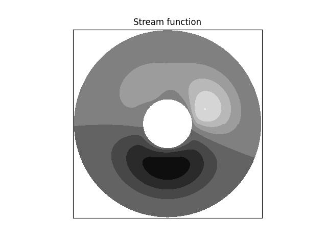
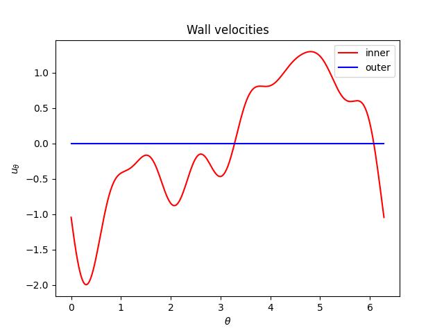
The results are displayed below.