Numerical Treatment

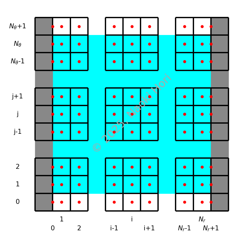
Let \(c_{i, j}\) be the concentration field, where the indices \(i\) and \(j\) denote the spatial locations in the radial and azimuthal directions, respectively. The index ranges are \(i = 0, 1, \dots, \nr, \nr + 1\) and \(j = 0, 1, \dots, \nt, \nt + 1\), where \(i = 0, \nr + 1\) and \(j = 0, \nt + 1\) store the boundary values and reflect periodicity, respectively. The following diagram illustrates the positioning of the concentration field \(c_{i, j}\) (reddish dots).

Below we briefly discuss the process to integrate the concentration field in time numerically. We assume that \(c_{i, j}^n\), a concentration field at step \(n\), is given.

Step 1: Computing the Stream Function

To start, from \(c\) on the particle surface (at \(\vr = 1\), or equivalently \(i = 0\)), we transform it to the spectral domain:

\[C_k^s \equiv \sum_{j = 0}^{\nt - 1} c_{0, j + 1} \expp{- \frac{j k}{\nt} I},\]

where \(k = 0, 1, \dots, \nt - 1\). Note that, because of \(c_{i, j} \in \mathbb{R}\), \(C_k^s\) satisfies the complex-conjugate property:

\[C_k^s = \left( C_{\nt - k}^s \right)^*\]

for \(k = 1, 2, \dots, \nt / 2 - 1\). Additionally, \(C_0^s\) and \(C_{\nt / 2}^s\) are real numbers.

Since the concentration \(c\) is located at cell centers in the azimuthal direction, we need to apply a half-grid shift azimuthally, which is achieved by modifying the argument:

\[{C_k^s}^\prime \equiv C_k^s \expp{- \pi \frac{k}{\nt} I}.\]

Using \({C_k^s}^\prime\), the azimuthal velocity on the particle is obtained by:

\[\vat{\ut}{r = 1} = \vat{ \frac{1}{\vr} \pder{}{c}{\vt} }{ r = 1 },\]

or in the frequency domain:

\[\vat{U_\vt}{r = 1} \equiv U_{\vt}^s = I k {C_k^s}^\prime.\]

Finally we evaluate the stream function in the frequency domain at radial cell faces \(\Psi_{i + \frac{1}{2}, k}\). The inverse transform of \(\Psi_{i + \frac{1}{2}, k}\) yields \(\psi_{i + \frac{1}{2}, j + \frac{1}{2}}\), defined at cell corners.

Step 2: Computing Staggered Velocity

To ensure conservative transport of the concentration field, the velocity components are positioned in a staggered manner. Since the stream function \(\psi\) is defined at cell corners, the staggered velocity components are computed as:

\[\vat{\ur}{i + \frac{1}{2}, j} = \frac{1}{\vr_{i + \frac{1}{2}}} \vat{\dder{}{\psi}{\vt}}{i + \frac{1}{2}, j},\]

\[\vat{\ut}{i, j + \frac{1}{2}} = - \vat{\dder{}{\psi}{\vr}}{i, j + \frac{1}{2}}.\]

Note

Regardless of how the stream function \(\psi\) is specified, the discrete incompressibility constraint evaluated at cell centers:

\[\frac{1}{\vr} \dder{}{}{\vr} \left( \vr \dder{}{\ur}{\vr} \right) + \frac{1}{\vr} \dder{}{}{\vt} \left( \dder{}{\ut}{\vt} \right) = 0, \,\, \forall \left( i, j \right)\]

is always satisfied.

Step 3: Transporting the Concentration

Since the concentration field is located at cell centers and is surrounded by staggered velocity components, we update \(c\) using the standard approach:

\[ \begin{align}\begin{aligned}\pder{}{\scalar}{t} = & - \dscalaradv{1}{\scalar} - \dscalaradv{2}{\scalar}\\& + \frac{1}{Pe} \dscalardif{1}{\scalar} + \frac{1}{Pe} \dscalardif{2}{\scalar}.\end{aligned}\end{align} \]

The radial boundary conditions read

\[\frac{ 1 }{ \vat{\sfact{1}}{r = 1} } \left( c_{1, j} - c_{0, j} \right) = -1 \quad \Leftrightarrow \quad c_{0, j} = c_{1, j} + \vat{\sfact{1}}{r = 1}\]

and

\[c_{\nr + 1, j} = 0.\]

See also

Refer to SimpleTCSolver for detailed derivation.

The above scheme is first-order accurate in time, which is not sufficient practically. Also, it is advantageous to treat the diffusive terms implicitly in time to eliminate the severe time-step constraint. To circumvent these obstacles, here we adopt the third-order Runge-Kutta scheme to improve the temporal accuracy. Each sub step denoted by the superscript \(n\) is given by:

\[ \begin{align}\begin{aligned}& h^n = \left( adv. \right)^n + \beta^n h^{n - 1},\\& \left( \Delta c \right) - \eta \alpha^n \Delta t \left[ \frac{1}{Pe} \dscalardif{1}{\left( \Delta \scalar \right)} + \frac{1}{Pe} \dscalardif{2}{\left( \Delta \scalar \right)} \right]\\& \quad = \gamma^n \Delta t h^n + \alpha^n \Delta t \left[ \frac{1}{Pe} \dscalardif{1}{\scalar^n} + \frac{1}{Pe} \dscalardif{2}{\scalar^n} \right]\\& \quad \equiv \left( rhs \right)^n,\\& c^{n + 1} = c^n + \left( \Delta c \right),\end{aligned}\end{align} \]

where \(\left( adv. \right)\) represents the sum of the two advective terms:

\[\left( adv. \right)^n \equiv - \dscalaradv{1}{\scalar^n} - \dscalaradv{2}{\scalar^n}.\]

The parameter \(\eta\) is a constant that controls the implicitness of the scheme. Typically, we use \(\eta = 1 / 2\) to achieve a second-order accurate semi-implicit (Crank-Nicolson) scheme or \(\eta = 1\) for a first-order accurate fully implicit scheme.

The Runge-Kutta coefficients are (Williamson, J. Comput. Phys. (35), 1980):

\[\begin{split}\begin{array}{c|ccc} & 0 & 1 & 2 \\ \hline \alpha & \frac{+1920}{5760} & \frac{+2400}{5760} & \frac{+1440}{5760} \\ \beta & \frac{ 0}{5760} & \frac{-3200}{5760} & \frac{-6885}{5760} \\ \gamma & \frac{+1920}{5760} & \frac{+5400}{5760} & \frac{+3072}{5760} \\ \end{array}\end{split}\]

To simplify the discrete Helmholtz operator on the left-hand side, we focus on the azimuthal component of the discrete Laplace operator with respect to a cell-centered quantity \(q\):

\[\dscalardif{2}{q}.\]

Since neither the azimuthal scale factor \(\sfact{2}\) nor the Jacobian determinant \(J\) varies in the azimuthal direction, we can extract the pre-factors from the discrete divergence operator, yielding

\[\frac{1}{\sfact{2}} \frac{1}{\sfact{2}} \dif{ }{\gcs{2}} \dif{q}{\gcs{2}}.\]

Now, we evaluate this quantity at a cell center \(\left( i, j \right)\). Given that the azimuthal grid is equidistant, we expand \(q\) using a discrete Fourier series:

\[q_{i, j} = \sum_l Q_{i, l} \expp{2 \pi \frac{j l}{\nt} I}.\]

Since neighboring cell centers yield

\[q_{i, j \pm 1} = \sum_l Q_{i, l} \expp{2 \pi \frac{j l}{\nt} I} \expp{\pm 2 \pi \frac{l}{\nt} I},\]

it follows that

\[\frac{1}{\sfact{2}} \frac{1}{\sfact{2}} \dif{ }{\gcs{2}} \dif{q}{\gcs{2}} = \frac{1}{\sfact{2}} \frac{1}{\sfact{2}} \sum_l \left[ - 4 \sin^2 \left( \pi \frac{l}{\nt} \right) \right] Q_{i, l} \expp{2 \pi \frac{j l}{\nt} I}.\]

As a result, the main equation becomes

\[ \begin{align}\begin{aligned}\sum_l \left[ \left( \Delta C \right)_{i, l} - \frac{\eta \alpha^n \Delta t}{Pe} \dscalardif{1}{\left( \Delta C \right)_{i, l}} + 4 \sin^2 \left( \pi \frac{l}{\nt} \right) \frac{\eta \alpha^n \Delta t}{Pe} \frac{1}{\sfact{2}} \frac{1}{\sfact{2}} \left( \Delta C \right)_{i, l} \right] \expp{2 \pi \frac{j l}{\nt} I}\\= \sum_l \left( RHS \right)_{i, l} \expp{2 \pi \frac{j l}{\nt} I},\end{aligned}\end{align} \]

where \(\left( \Delta C \right)_{i, k}\) and \(\left( RHS \right)_{i, l}\) denote the Fourier coefficients of \(\left( \Delta c \right)\) and the right-hand side, respectively.

By applying the forward transform to both sides:

\[\sum_k \left[ \sum_l \left( RHS \right)_{i, l} \expp{2 \pi \frac{j l}{\nt} I} \right] \expp{- 2 \pi \frac{j k}{\nt} I},\]

we obtain

\[\left[ 1 + \frac{4 \eta \alpha^n \Delta t}{Pe} \left\{ \frac{1}{\sfact{2}} \sin \left( \pi \frac{k}{\nt} \right) \right\}^2 \right] \left( \Delta C \right)_{i, k} - \frac{\eta \alpha^n \Delta t}{Pe} \dscalardif{1}{\left( \Delta C \right)_{i, k}} = \left( RHS \right)_{i, k}.\]

Since no terms involve \(k \pm 1\), this results in a purely tri-diagonal linear system in the radial direction for each azimuthal wave number \(k\).

Regarding the radial boundary conditions, because of

\[c_{0, j}^{n + 1} = c_{1, j}^{n + 1} + \vat{\sfact{1}}{r = 1}\]

and

\[c_{0, j}^n = c_{1, j}^n + \vat{\sfact{1}}{r = 1},\]

we have

\[\left( \Delta c \right)_{0, j} = \left( \Delta c \right)_{1, j}\]

or in the azimuthal spectral space:

\[\left( \Delta C \right)_{0, k} = \left( \Delta C \right)_{1, k},\]

giving a zero Neumann boundary condition on the particle surface. On the outer circle where a Dirichlet condition is imposed, we simply have

\[\left( \Delta C \right)_{\nr + 1, k} = 0.\]