Cartesian coordinates

The biharmonic equation in Cartesian coordinates is written explicitly as:

\[\newcommand{\vx}{x} \newcommand{\vy}{y} \newcommand{\lx}{L_{\vx}} \newcommand{\ly}{L_{\vy}} \newcommand{\ux}{u_{\vx}} \newcommand{\uy}{u_{\vy}} \pder{4}{\psi}{\vx} + 2 \pder{2}{}{\vx} \pder{2}{\psi}{\vy} + \pder{4}{\psi}{\vy} = 0.\]

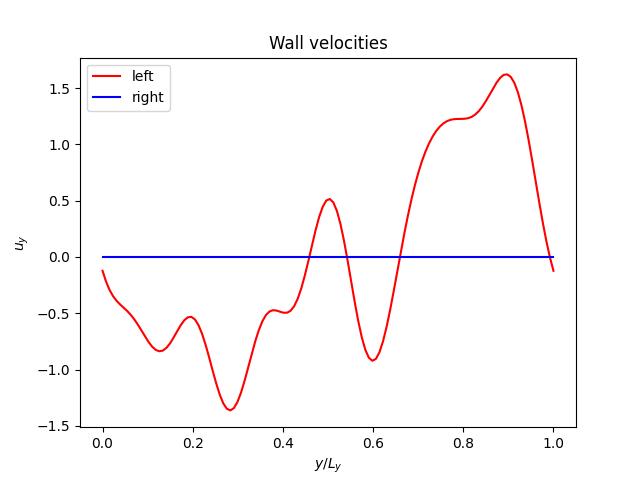
The domain is wall-bounded in the \(x\) direction. The boundary conditions on the walls are

\[ \begin{align}\begin{aligned}\ux & = \pder{}{\psi}{\vy} = 0,\\\uy & = - \pder{}{\psi}{\vx} = f_{\pm} \left( \vy \right),\end{aligned}\end{align} \]

where \(f_{\pm} \left( \vy \right)\) represents the prescribed wall velocities.

Using the Fourier series, \(\psi\) reads

\[\psi \left( \vx, \vy \right) = \sum_k \Psi_k \left( \vx \right) \expp{I k \vy},\]

where \(I\) is the imaginary unit and \(k \equiv 2 \pi k^\prime / \ly\) with \(k^\prime \in \mathbb{Z}\) being the wave number.

Substituting this relation into the biharmonic equation yields:

\[\sum_k \left( k^4 \Psi_k - 2 k^2 \der{2}{\Psi_k}{\vx} + \der{4}{\Psi_k}{\vx} \right) \expp{I k \vy} = 0.\]

Due to the orthogonality of the trigonometric functions, we obtain

\[\der{4}{\Psi_k}{\vx} - 2 k^2 \der{2}{\Psi_k}{\vx} + k^4 \Psi_k = 0.\]

Since the characteristic equation of this differential equation:

\[\lambda^4 - 2 k^2 \lambda^2 + k^4 = 0\]

has the roots:

\[\lambda = \pm k,\]

the homogeneous solution leads to

\[\Psi_k = A_k \expp{kx} + B_k \vx \expp{kx} + C_k \expp{- kx} + D_k \vx \expp{- kx},\]

and its wall-normal derivative:

\[\der{}{\Psi_k}{\vx} = A_k k \expp{k \vx} + B_k \left( 1 + k \vx \right) \expp{k \vx} + C_k \left( - k \right) \expp{- k \vx} + D_k \left( 1 - k \vx \right) \expp{- k \vx}.\]

The coefficients \(A_k, B_k, C_k, D_k\) are determined from the boundary conditions:

\[\ux = \pder{}{\psi}{\vy} = \sum_k I k \Psi_k \expp{I k \vy} = 0,\]

\[\uy = - \pder{}{\psi}{\vx} = - \sum_k \der{}{\Psi_k}{\vx} \expp{I k \vy} = f_{\pm} \left( \vy \right),\]

or equivalently:

\[I k \Psi_k = 0,\]

\[\der{}{\Psi_k}{\vx} = - \int f_{\pm} \left( \vy \right) \expp{- I k \vy} d \vy.\]

The second relation is simply the Fourier transform of the prescribed wall velocities with the sign flipped, while the first relation states that

\[\Psi_k = 0\]

for \(k \ne 0\), while \(k = 0\) imposes no condition, as we only enforce Neumann conditions with respect to \(\psi\).

The implementation is as follows.

def compute_stream_function(xs: np.ndarray, ys: np.ndarray, bc: [np.ndarray, np.ndarray]) -> np.ndarray:
    # convert wall velocities to frequency domain
    uy_m = - np.fft.rfft(bc[0])
    uy_p = - np.fft.rfft(bc[1])
    # compute stream function in frequency domain
    psi_freq = np.zeros((ny // 2 + 1, nx), dtype="complex128")
    mat = np.zeros((4, 4), dtype="float64")
    vec = np.zeros((4), dtype="complex128")
    # zero-th mode cannot be determined: just assign zero
    psi_freq[0, :] = 0
    for k in range(1, ny // 2 + 1):
        # for each wavenumber, compute coefficients
        mat[0] = get_f(k, xlim[0])
        mat[1] = get_f(k, xlim[1])
        mat[2] = get_dfdx(k, xlim[0])
        mat[3] = get_dfdx(k, xlim[1])
        vec[0] = 0
        vec[1] = 0
        vec[2] = uy_m[k]
        vec[3] = uy_p[k]
        coefs = np.linalg.solve(mat, vec)
        # for each wall-normal position, compute stream function
        for i, x in enumerate(xs):
            psi_freq[k, i] = np.dot(coefs, get_f(k, x))
    # convert frequency domain to physical domain
    psi = np.zeros((ny, nx), dtype="float64")
    for i, x in enumerate(xs):
        psi[:, i] = np.fft.irfft(psi_freq[:, i])
    return psi

def compute_boundary_condition(ys: np.ndarray) -> [np.ndarray, np.ndarray]:
    uy_m = np.zeros(ys.shape)
    uy_p = np.zeros(ys.shape)
    for k in range(1, 8):
        amp = np.power(float(k), -1)
        phase = 2 * np.pi * np.random.random_sample()
        uy_m += amp * np.sin(2 * np.pi * (k * ys / (ylim[1] - ylim[0]) + phase))
    return uy_m, uy_p

def get_f(k: float, x: float) -> float:
    return [
        1 * np.exp(+ k * x),
        x * np.exp(+ k * x),
        1 * np.exp(- k * x),
        x * np.exp(- k * x),
    ]

def get_dfdx(k: float, x: float) -> float:
    return [
        (0 + k * 1) * np.exp(+ k * x),
        (1 + k * x) * np.exp(+ k * x),
        (0 - k * 1) * np.exp(- k * x),
        (1 - k * x) * np.exp(- k * x),
    ]

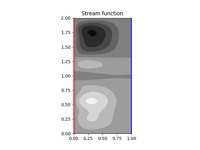
The computed stream function under

\[ \begin{align}\begin{aligned}\lx & = 1,\\\ly & = 2,\\f_{-} \left( \vy \right) & = \sum_{k = 1}^8 k^{-1} \sin \left( 2 \pi k \frac{\vy}{\ly} + \varphi_k \right),\\f_{+} \left( \vy \right) & = 0\end{aligned}\end{align} \]

is shown below: