Surface normal

Overview

I assume that I know the profile of \(\phi\) at step \(n\), e.g.

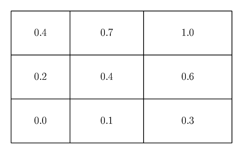
Discrete phase distribution (volume fraction) in a two-dimensioinal domain.

Note

In this project, uniform grid spacings are adopted in the homogeneous (\(y\)) direction(s), while non-uniform grids can be used in the wall-normal (\(x\)) direction.

In the above figure, the left-bottom and the right-top cells are fully occupied by one of the two phases, while two liquids coexist in the other cells.

To start the surface reconstruction, I first compute the local surface normal. In particular, I would like to compute the local normal vector defined at each cell center \(n_{\pic,\pjc}\).

There are many options, depending on the accuracy required and the computational cost. Here, I adopt one of the most simple approaches using the fact that the surface normal is given by

\[n_i = \frac{m_i}{\left| m_i \right|},\]

where \(m_i\) is the local gradient of the indicator function and is approximated as

\[m_i \approx \der{\phi}{x_i}.\]

To compute this quantity at the cell center \(\left( \pic, \pjc \right)\), one of the easiest ways would be to use the second-order-accurate central-difference scheme:

\[\der{\phi}{x} \approx \frac{\phi_{\pipp, \pjc} - \phi_{\pimm, \pjc}}{2 \Delta x},\]

which tends to be unstable since this skips \(\phi_{\pic, \pjc}\) to evaluate the derivative there (not diagonally-dominant).

Instead, I adopt the Youngs approach (introduced by Youngs, Numer. Methods Fluid Dyn., 1982, extensively explained by Ii et al., J. Comput. Phys. (231), 2012), which is discussed in the following section.

Youngs approach

1. Compute gradients at the cell corners

   To begin with, I compute the gradients at the cell corners (not the center). I use 4 (or 9 in 3D) surrounding cells to compute the gradients at the cell corners.

   Gradients in the \(x\) direction:

   \[\begin{split}\vat{m_x}{\pim, \pjm} & \approx \vat{\der{\phi}{x}}{\pim, \pjm}, \\ \vat{m_x}{\pip, \pjm} & \approx \vat{\der{\phi}{x}}{\pip, \pjm}, \\ \vat{m_x}{\pim, \pjp} & \approx \vat{\der{\phi}{x}}{\pim, \pjp}, \\ \vat{m_x}{\pip, \pjp} & \approx \vat{\der{\phi}{x}}{\pip, \pjp}.\end{split}\]
   src/interface/curvature_tensor.c

   const double dx = DXC(i  );
   const double dvofdx = 1. / dx * (
       - VOF(i-1, j-1) + VOF(i  , j-1)
       - VOF(i-1, j  ) + VOF(i  , j  )
   );
   

   src/interface/curvature_tensor.c

   const double dvofdx = 1. / dx * (
       - VOF(i-1, j-1, k-1) + VOF(i  , j-1, k-1)
       - VOF(i-1, j  , k-1) + VOF(i  , j  , k-1)
       - VOF(i-1, j-1, k  ) + VOF(i  , j-1, k  )
       - VOF(i-1, j  , k  ) + VOF(i  , j  , k  )
   );
   

   Gradients in \(y\):

   \[\begin{split}\vat{m_y}{\pim, \pjm} & \approx \vat{\der{\phi}{y}}{\pim, \pjm}, \\ \vat{m_y}{\pip, \pjm} & \approx \vat{\der{\phi}{y}}{\pip, \pjm}, \\ \vat{m_y}{\pim, \pjp} & \approx \vat{\der{\phi}{y}}{\pim, \pjp}, \\ \vat{m_y}{\pip, \pjp} & \approx \vat{\der{\phi}{y}}{\pip, \pjp}.\end{split}\]
   src/interface/curvature_tensor.c

   const double dvofdy = 1. / dy * (
       - VOF(i-1, j-1) - VOF(i  , j-1)
       + VOF(i-1, j  ) + VOF(i  , j  )
   );
   

   src/interface/curvature_tensor.c

   const double dvofdy = 1. / dy * (
       - VOF(i-1, j-1, k-1) - VOF(i  , j-1, k-1)
       + VOF(i-1, j  , k-1) + VOF(i  , j  , k-1)
       - VOF(i-1, j-1, k  ) - VOF(i  , j-1, k  )
       + VOF(i-1, j  , k  ) + VOF(i  , j  , k  )
   );
   

   Gradients in \(z\):

   src/interface/curvature_tensor.c

   const double dvofdz = 1. / dz * (
       - VOF(i-1, j-1, k-1) - VOF(i  , j-1, k-1)
       - VOF(i-1, j  , k-1) - VOF(i  , j  , k-1)
       + VOF(i-1, j-1, k  ) + VOF(i  , j-1, k  )
       + VOF(i-1, j  , k  ) + VOF(i  , j  , k  )
   );
   

   Note that they are gradients and not the normal vectors. To obtain normal, I normalise them and the results are assigned to the resulting array DVOF.

   src/interface/curvature_tensor.c

   const double norm = sqrt(
       + pow(dvofdx, 2.)
       + pow(dvofdy, 2.)
   );
   const double norminv = 1. / fmax(norm, DBL_EPSILON);
   DVOF(i, j)[0] = dvofdx * norminv;
   DVOF(i, j)[1] = dvofdy * norminv;
   

   src/interface/curvature_tensor.c

   const double norm = sqrt(
       + pow(dvofdx, 2.)
       + pow(dvofdy, 2.)
       + pow(dvofdz, 2.)
   );
   const double norminv = 1. / fmax(norm, DBL_EPSILON);
   DVOF(i, j, k)[0] = dvofdx * norminv;
   DVOF(i, j, k)[1] = dvofdy * norminv;
   DVOF(i, j, k)[2] = dvofdz * norminv;
   

   

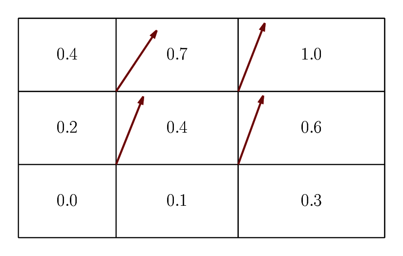
   Normal vectors at the surrounding cell corners.

   Note

   In this image, lengths of the arrows are adjusted for the sake of appearance and thus may be inaccurate.

2. Compute normals at the cell centers

   The normal vector defined at each cell center is computed by averaging the normals defined at the surrounding cell corners:

   src/interface/curvature_tensor.c

   double nx = (
       + DVOF(i  , j  )[0] + DVOF(i+1, j  )[0]
       + DVOF(i  , j+1)[0] + DVOF(i+1, j+1)[0]
   );
   

   src/interface/curvature_tensor.c

   double nx = (
       + DVOF(i  , j  , k  )[0] + DVOF(i+1, j  , k  )[0]
       + DVOF(i  , j+1, k  )[0] + DVOF(i+1, j+1, k  )[0]
       + DVOF(i  , j  , k+1)[0] + DVOF(i+1, j  , k+1)[0]
       + DVOF(i  , j+1, k+1)[0] + DVOF(i+1, j+1, k+1)[0]
   );
   

   src/interface/curvature_tensor.c

   double ny = (
       + DVOF(i  , j  )[1] + DVOF(i+1, j  )[1]
       + DVOF(i  , j+1)[1] + DVOF(i+1, j+1)[1]
   );
   

   src/interface/curvature_tensor.c

   double ny = (
       + DVOF(i  , j  , k  )[1] + DVOF(i+1, j  , k  )[1]
       + DVOF(i  , j+1, k  )[1] + DVOF(i+1, j+1, k  )[1]
       + DVOF(i  , j  , k+1)[1] + DVOF(i+1, j  , k+1)[1]
       + DVOF(i  , j+1, k+1)[1] + DVOF(i+1, j+1, k+1)[1]
   );
   

   src/interface/curvature_tensor.c

   double nz = (
       + DVOF(i  , j  , k  )[2] + DVOF(i+1, j  , k  )[2]
       + DVOF(i  , j+1, k  )[2] + DVOF(i+1, j+1, k  )[2]
       + DVOF(i  , j  , k+1)[2] + DVOF(i+1, j  , k+1)[2]
       + DVOF(i  , j+1, k+1)[2] + DVOF(i+1, j+1, k+1)[2]
   );
   

   

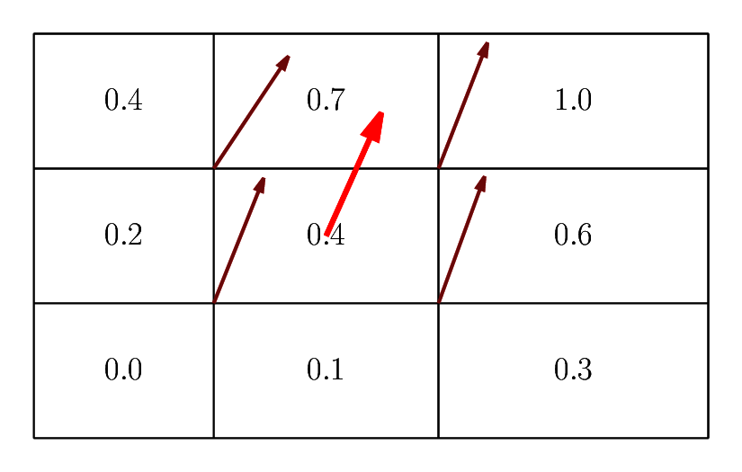
   Normal vector at the cell center.

   Note

   In this image, lengths of the arrows are adjusted for the sake of appearance and thus may be inaccurate. In general, the norm of the new vector is not unity.

3. Coordinate transformation

   The normal vector at each cell center is defined on the global coordinate system (e.g., coordinate system used to describe the domain), whose basis is \(\left( \underline{e}_x, \underline{e}_y \right)\). For convenience, I define a local coordinate system which is attached to each cell \(\left( i, j \right)\), whose basis is \(\left( \underline{e}_{X}, \underline{e}_{Y} \right)\). These two coordinate systems are related with

   \[\begin{split}\begin{pmatrix} \underline{e}_X \\ \underline{e}_Y \end{pmatrix} = \begin{pmatrix} \Delta x_i & 0 \\ 0 & \Delta y \end{pmatrix} \begin{pmatrix} \underline{e}_x \\ \underline{e}_y \end{pmatrix},\end{split}\]

   or equivalently

   \[\begin{split}\begin{pmatrix} \underline{e}_x \\ \underline{e}_y \end{pmatrix} = \begin{pmatrix} \frac{1}{\Delta x_i} & 0 \\ 0 & \frac{1}{\Delta y} \end{pmatrix} \begin{pmatrix} \underline{e}_X \\ \underline{e}_Y \end{pmatrix}.\end{split}\]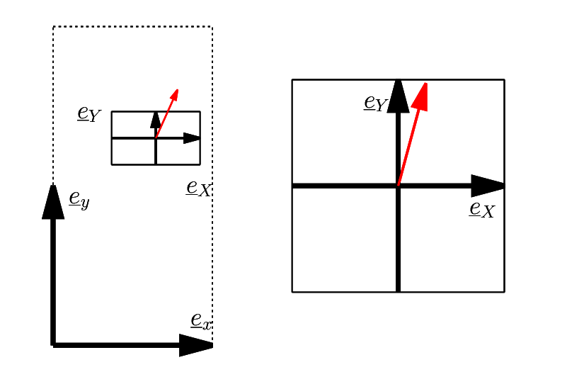

   

   (Left) global coordinate system, and (right) local coordinate system used in this project. Notice that the directions of the reddish arrows differ, which is because the grid size is scaled.

   Thus, the above normal vector defined on the globa* coordinate system

   \[n_i^{global} = \underline{e}_x n_x + \underline{e}_y n_y\]

   is written as

   \[\underline{e}_X \frac{1}{\Delta x_i} n_x + \underline{e}_Y \frac{1}{\Delta y } n_y\]

   on the local coordinate system.

   Finally, the surface normal defined at the cell center of the local coordinate system is computed as

   \[n_i^{local} \equiv \underline{e}_X n_X + \underline{e}_Y n_Y,\]

   which is

   \[\begin{split}n_X &= \frac{1}{k} \frac{n_x}{\Delta x_{i}}, \\ n_Y &= \frac{1}{k} \frac{n_y}{\Delta y },\end{split}\]

   where

   \[k \equiv \sqrt{ \left( \frac{n_x}{\Delta x_{i}} \right)^2 + \left( \frac{n_y}{\Delta y } \right)^2 }.\]
   src/interface/curvature_tensor.c

   nx /= dx;
   ny /= dy;
   const double norm = sqrt(
       + pow(nx, 2.)
       + pow(ny, 2.)
   );
   const double norminv = 1. / fmax(norm, DBL_EPSILON);
   nx *= norminv;
   ny *= norminv;
   

   src/interface/curvature_tensor.c

   nx = nx / dx;
   ny = ny / dy;
   nz = nz / dz;
   const double norm = sqrt(
       + pow(nx, 2.)
       + pow(ny, 2.)
       + pow(nz, 2.)
   );
   const double norminv = 1. / fmax(norm, DBL_EPSILON);
   nx *= norminv;
   ny *= norminv;
   nz *= norminv;
   

Note

On the new coordinate system, each control volume is a unit square.