Intercept and THINC scheme

Overview

In the previous section, the surface normal is computed at each cell center. This information is, however, not enough to uniquely define the surface position uniquely:

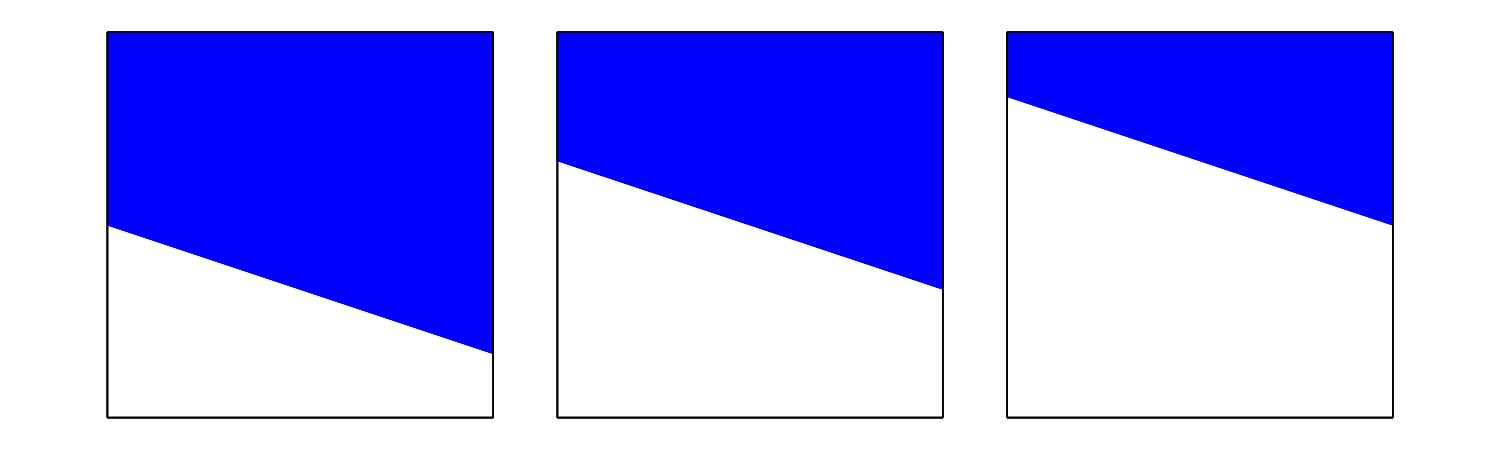
Three different interfacial positions having the same surface normal.

In this image, for example, although all three surface patterns have the same surface normal, they are obviously different.

Since the three cases have the different occupations, I use the information to fix the surface position:

\[\frac{1}{V_{ij}} \int_{V_{ij}} H dV_{ij} = \phi_{ij},\]

which is the definition of \(\phi\).

Note

In the previous section, I defined local coordinate systems such that the size of the computational cells \(V_{ij}\) is \(1\). The origin of the local coordinates locates at the cell center, and as a result the cell edges exist at \(x = \pm \frac{1}{2}\) and \(y = \pm \frac{1}{2}\).

Mathematically or physically speaking, since the free surface is discontinuous, \(H\) is a step function. Conventional VOF methods solve the equation based on this assumption.

In this project, I treat this problem in a different way here: instead of \(H\) (step function), I consider a slightly smoothed function \(\hat{H}\):

\[\begin{split}H \left( n_X X + n_Y Y + d \right) & \approx \hat{H} \left( n_X X + n_Y Y + d \right) \\ & \equiv \frac{1}{2} \left[ 1 + \tanh \left\{ \beta \left( n_X X + n_Y Y + d \right) \right\} \right].\end{split}\]

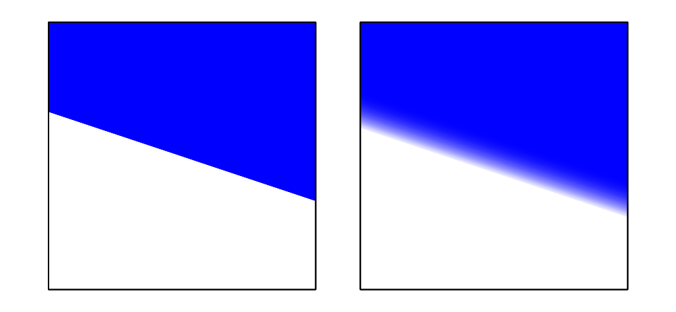
Sharp (left, \(H \left( x, y \right)\)) and smoothed (right, \(\hat{H} \left( x, y \right)\)) interfacial representations.

\(d\) is a parameter to be defined here, giving the surface position. \(\beta\) is a sharpness parameter which specifies the thickness, which corresponds to the Cahn number \(Cn\) in the phase-field methods:

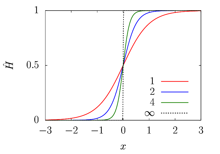
Interface sharpness as a function of the control parameter \(\beta\). \(\beta \rightarrow \infty\) leads to \(H\). \(\Delta x = 1\) corresponds to the size of the grid.

Note

The larger the \(\beta\) is, the sharper the surface becomes and the more realistic it is. However, there are two drawbacks for large \(\beta\):

• Inaccurate surface representation

  As discussed below, the numerical integral of \(\hat{H}\) is justified by the fact that \(\hat{H}\) is smooth. Larger \(\beta\) violates this assumption, and higher-order Gaussian quadratures are needed to accurately compute the surface position, which is computationally demanding.

• Large spurious currents

  THINC schemes tend to suppress the spurious currents well compared to the conventional VOF method, which comes from the diffused nature of the surface. Larger \(\beta\) diminishes this advantage.

Recall that here I want to decide \(d\) to uniquely decide the position of the local surface. Although the above equation has an analytical solution for two-dimensional cases, it contains Eulerian logarithmic integrals, which is computationally expensive. Thanks to the diffused assumption of the surface, however, numerical integral gives a good approximation, namely:

\[\int_{V} \hat{H} \left( n_X X + n_Y Y + d \right) dV \approx \sum_{i}^N \sum_{j}^N w_i w_j \hat{H} \left( n_X X_i + n_Y Y_j + d \right) = \phi,\]

where \(w_i\) and \(X_i\) are the weights and the points of \(N\)-th-order Gaussian quadrature defined in the interval \(\left[ -\frac{1}{2}, +\frac{1}{2} \right]\). Notice that the volume integral is replaced with the summations in all dimensions.

To obtain \(d\), I need to minimise the following function \(f\):

\[f \left( d \right) \equiv - \phi + \sum_{i}^N \sum_{j}^N w_i w_j \hat{H} \left( n_X X_i + n_Y Y_j + d \right).\]

For simplicity, I introduce

\[\psi \equiv \psi \left( X, Y \right) \equiv n_X X + n_Y Y.\]

here. Also I use an identity:

\[\hat{H} \left( x \right) = \frac{1}{2} \left\{ 1 + \tanh \left( x \right) \right\} \equiv \frac{1}{1 + \exp{\left( - 2 \beta x \right)}},\]

to yield

\[f \left( d \right) \equiv - \phi + \sum_{i}^N \sum_{j}^N \frac{w_i w_j}{ 1 + \exp{ \left\{ - 2 \beta \left( \psi + d \right) \right\} } }.\]

Since \(\exp{\left( x \right)}\) is a monotonic function, finding \(d\) is equivalent to finding the corresponding \(D \equiv \exp{\left(-2 \beta d \right)}\):

\[f \left( D \right) \equiv - \phi + \sum_{i}^N \sum_{j}^N \frac{w_i w_j}{ 1 + P_{ij} D },\]

and its derivative (with respect to \(D\) instead of \(d\)) is

\[f^{\prime} \left( D \right) \equiv \sum_{i}^N \sum_{j}^N \frac{- w_i w_j P_{ij}}{ \left( 1 + P_{ij} D \right)^2 },\]

where

\[P_{ij} \equiv \exp{\left( - 2 \beta \psi_{ij} \right)}.\]

Newton-Raphson method

Roughly speaking, to obtain \(d\) (or \(D\)), I move the hyper-surface (see below) and find \(d\), whose (numerical) integral coincides with the given local volume fraction \(\phi\).

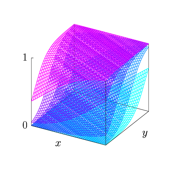
Hyper-surfaces \(\hat{H} \left( x, y, d \right)\) as a function of \(d\), while the normal vector is fixed.

which is achieved by the Newton-Raphson method following Xie and Xiao, J. Comput. Phys. (349), 2017.

Notice that \(P_{ij} = \exp{\left( -2\beta \psi_{ij} \right)}\) is independent of \(D\) and thus I compute them before starting the iteration:

src/interface/curvature_tensor.c

double exps[NGAUSS * NGAUSS] = {0.};
for(int jj = 0; jj < NGAUSS; jj++){
  for(int ii = 0; ii < NGAUSS; ii++){
    exps[jj * NGAUSS + ii] = exp(
        -2. * vofbeta * (
          + normal[0] * gauss_ps[ii]
          + normal[1] * gauss_ps[jj]
        )
    );
  }
}

src/interface/curvature_tensor.c

double exps[NGAUSS * NGAUSS * NGAUSS] = {0.};
for(int kk = 0; kk < NGAUSS; kk++){
  for(int jj = 0; jj < NGAUSS; jj++){
    for(int ii = 0; ii < NGAUSS; ii++){
      exps[(kk * NGAUSS + jj) * NGAUSS + ii] = exp(
          -2. * vofbeta * (
            + normal[0] * gauss_ps[ii]
            + normal[1] * gauss_ps[jj]
            + normal[2] * gauss_ps[kk]
          )
      );
    }
  }
}

Also, to start the iteration, I need the initial \(D_0\). As a guess, I take the solution of the first-order Gaussian quadrature:

\[P_{00} = \exp{\left\{ \psi \left( X = 0, Y = 0 \right) \right\}} = 1\]

and

\[w_0 = 1,\]

giving

\[f \left( D_0 \right) = - \phi + \frac{1}{1 + D_0} = 0\]

and thus

\[D_0 = \frac{1}{\phi} - 1:\]

src/interface/curvature_tensor.c

double val = 1. / vof - 1.;

Also the function

\[f \left( D \right) \equiv - \phi + \sum_{i}^N \sum_{j}^N \frac{w_i w_j}{ 1 + P_{ij} D }\]

and its derivative

\[f^{\prime} \left( D \right) \equiv \sum_{i}^N \sum_{j}^N \frac{- w_i w_j P_{ij}}{ \left( 1 + P_{ij} D \right)^2 }\]

are computed here:

src/interface/curvature_tensor.c

    double f0 = -1. * vof;
    double f1 = 0.;
#if NDIMS == 2
    for(int jj = 0; jj < NGAUSS; jj++){
      for(int ii = 0; ii < NGAUSS; ii++){
        const double weight = gauss_ws[ii] * gauss_ws[jj];
        const double p = exps[jj * NGAUSS + ii];
        const double denom = 1. / (1. + p * val);
        f0 += weight     * denom;
        f1 -= weight * p * denom * denom;
      }
    }
#else
    for(int kk = 0; kk < NGAUSS; kk++){
      for(int jj = 0; jj < NGAUSS; jj++){
        for(int ii = 0; ii < NGAUSS; ii++){
          const double weight = gauss_ws[ii] * gauss_ws[jj] * gauss_ws[kk];
          const double p = exps[(kk * NGAUSS + jj) * NGAUSS + ii];
          const double denom = 1. / (1. + p * val);
          f0 += weight     * denom;
          f1 -= weight * p * denom * denom;
        }
      }
    }
#endif

\(D\) is updated using the computed \(f\) and \(f^{\prime}\):

\[D_{n+1} \leftarrow D_{n} - \frac{f}{f^{\prime}},\]

which is implemented as

src/interface/curvature_tensor.c

val -= f0 / f1;

This iteration continues until the residual \(| f |\) becomes smaller than the given threshold or until the number of iterations exceeds the specified maximum:

src/interface/curvature_tensor.c

const int cntmax = 8;
const double resmax = 1.e-12;

Finally I convert \(D\) to \(d\) following \(D = \exp{\left( -2\beta d \right)} \Leftrightarrow d = -\frac{1}{2\beta} \log{\left( D \right)}\):

src/interface/curvature_tensor.c

return -0.5 / vofbeta * log(val);

In the next step, I use this uniquely-determined surface to evaluate the flux to integrate the advection equation.