Typical case

To check whether the code works properly, a low Reynolds number case is simulated to see the Taylor rolls.

Configuration

#!/bin/bash

set -e
set -x

# set initial condition, model half cylinder
cd initial_condition
make output && make datadel
is_curved=true \
lx=1.0e+0 \
ly=0.39269908169872414 \
lz=2.0e+0 \
glisize=64 \
gljsize=8 \
glksize=32 \
python3 main.py output
cd ..

# build and run
make output && make datadel && make all
timemax=4.0e+2 \
wtimemax=6.0e+2 \
log_rate=1.0e+0 \
save_rate=1.0e+2 \
save_after=0.0e+0 \
stat_rate=1.0e-1 \
stat_after=1.0e+2 \
coef_dt_adv=1. \
coef_dt_dif=1. \
Re=80. \
Pr=1. \
mpirun -n 2 --oversubscribe ./a.out initial_condition/output

# post process
mkdir artifacts
python3 \
  docs/source/example/typical/data/snapshot.py \
  $(find output/save -type d | sort | tail -n 1) \
  artifacts/snapshot.png
python3 \
  docs/source/example/typical/data/divergence.py \
  output/log/divergence.dat \
  artifacts/divergence.png
python3 \
  docs/source/example/typical/data/balance_main.py \
  $(find output/save -type d | sort | tail -n 1) \
  output/log/dissipation.dat \
  output/log/injection.dat \
  artifacts/balance_main.png
python3 \
  docs/source/example/typical/data/balance_dif.py \
  output/log/dissipation.dat \
  output/log/injection.dat \
  artifacts/balance_dif.png

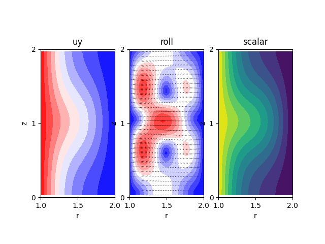
The azimuthal velocity field, radial-axial velocity field, and scalar field averaged in the azimuthal direction are visualised:

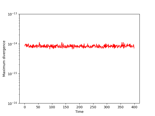
The maximum divergence as a function of time:

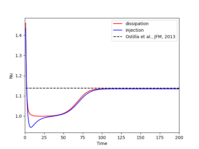
The normalised energy injection and dissipation (divided by the laminar reference value) inside the domain is plotted as a function of time. Note that these normalised energy budgets coincide with the definition of the Nusselt number of the angular velocity flux (Eckhardt et al., J. Fluid Mech. (581), 2007), and the black-dashed line is displayed as a counterpart (Ostilla et al., J. Fluid Mech. (719), 2013).

Recall that the schemes adopted in this project are designed so that the energy injection and the dissipation balances statistically, which can be confirmed by the following plot showing the difference between these two quantities as well as an analogous relation with respect to the passive scalar:

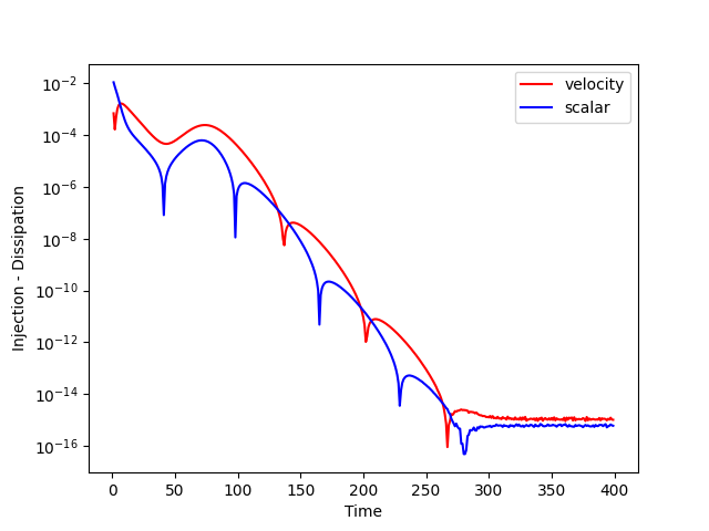
Initially they are different, which is because the flow is not in a steady state. Eventually the flow reaches a stationary state, at which the deviations vanish.