Equation

Boundary condition

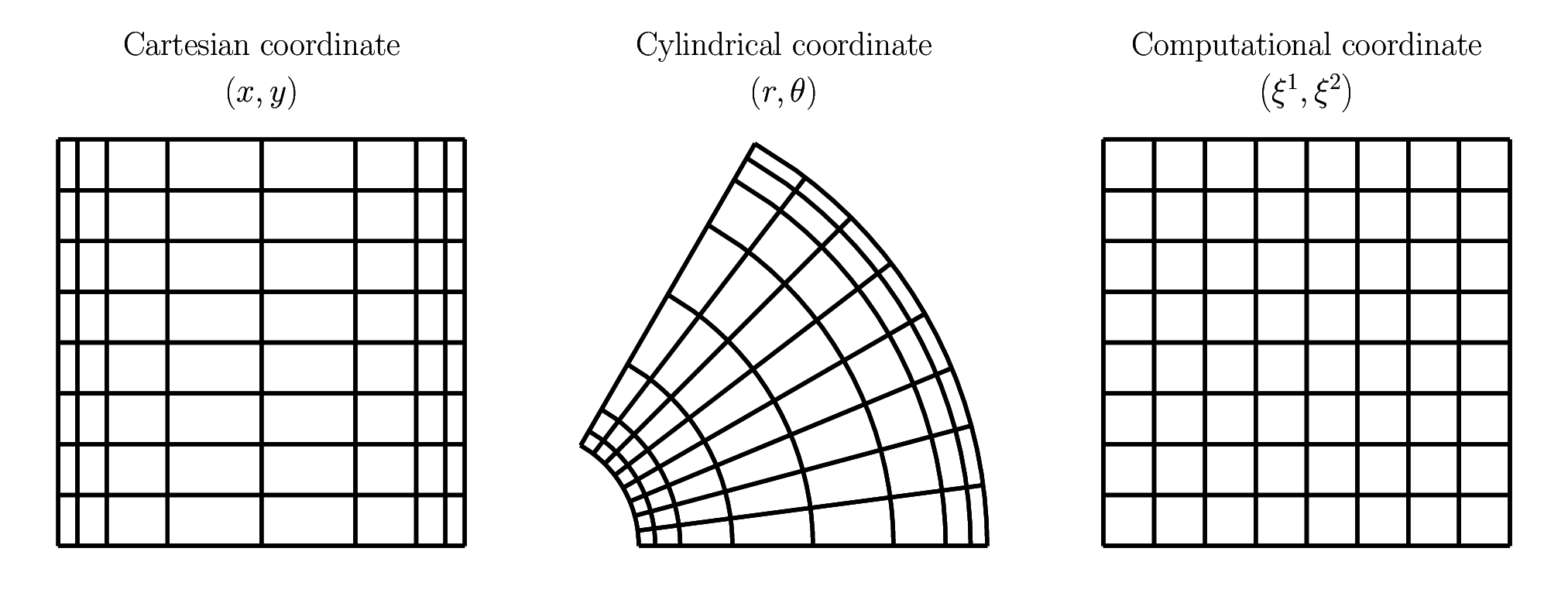
We focus on Cartesian (\(\vx,\vy,\vz\)) and cylindrical (\(\vr,\vt,\vz\)) domains which satisfy the following conditions.

• \(\vx, \vr\) directions are wall-bounded and impermeable condition is imposed.

• \(\vy, \vt\) directions are stream-wise, to which the walls may move with constant speeds over time and periodic boundary condition is imposed.

• \(\vz\) direction is span-wise, to which the walls do not move and periodic boundary condition is imposed.

Metric

For simplicity and generality, the governing equations are written in a general rectilinear coordinate system \(\gcs{i}\) with normalised components \(\vel{i}\) (c.f., Morinishi et al., J. Comput. Phys. (197), 2004). \(\sfact{i}\) denote scale factors and its product is the Jacobian determinant \(J\) due to the orthogonality.

There are several terms which are characteristic of cylindrical coordinates. In Cartesian coordinates, these additional terms lead to zero since \(\sfact{2}, \sfact{3}\) do not change in \(\gcs{1}\). Thus all equations, their numerical descriptions, and implementations can be unified.

See e.g., this for the derivations.

Shear-stress tensor

We define a second-order tensor representing the gradient of velocity vector:

\[\sum_i \sum_j \vec{e}_i \otimes \vec{e}_j \vgt{i}{j},\]

where the components \(\vgt{i}{j}\) are

\[\begin{split}\begin{pmatrix} \vgt{1}{1} & \vgt{2}{1} & \vgt{3}{1} \\ \vgt{1}{2} & \vgt{2}{2} & \vgt{3}{2} \\ \vgt{1}{3} & \vgt{2}{3} & \vgt{3}{3} \\ \end{pmatrix} = \begin{pmatrix} \frac{1}{\sfact{1}} \pder{\vel{1}}{\gcs{1}} & \frac{1}{\sfact{2}} \pder{\vel{1}}{\gcs{2}} - \frac{1}{J} \pder{}{\gcs{1}} \left( \frac{J}{\sfact{1}} \right) \vel{2} & \frac{1}{\sfact{3}} \pder{\vel{1}}{\gcs{3}} \\ \frac{1}{\sfact{1}} \pder{\vel{2}}{\gcs{1}} & \frac{1}{\sfact{2}} \pder{\vel{2}}{\gcs{2}} + \frac{1}{J} \pder{}{\gcs{1}} \left( \frac{J}{\sfact{1}} \right) \vel{1} & \frac{1}{\sfact{3}} \pder{\vel{2}}{\gcs{3}} \\ \frac{1}{\sfact{1}} \pder{\vel{3}}{\gcs{1}} & \frac{1}{\sfact{2}} \pder{\vel{3}}{\gcs{2}} & \frac{1}{\sfact{3}} \pder{\vel{3}}{\gcs{3}} \end{pmatrix}.\end{split}\]

The shear-stress tensor for Newtonian liquids is defined using the symmetric part of \(\vgt{i}{j}\):

\[\sst{i}{j} \equiv \mu \vgt{i}{j} + \mu \vgt{j}{i}.\]

Viscous contribution on the momentum balance is given by the divergence of this tensor:

\[\pder{}{x_j} \left( \mu \vgt{i}{j} + \mu \vgt{j}{i} \right).\]

Note that we assume \(\mu\) is constant in this project to obtain

\[\mu \pder{}{x_j} \left( \vgt{j}{i} + \vgt{i}{j} \right).\]

Hereafter we use kinematic viscosity \(\nu \equiv \mu / \rho\), since we assume the density \(\rho\) is constant as well.

Incompressibility constraint

\[\frac{1}{J} \pder{}{\gcs{1}} \left( \frac{J}{\sfact{1}} \vel{1} \right) + \frac{1}{J} \pder{}{\gcs{2}} \left( \frac{J}{\sfact{2}} \vel{2} \right) + \frac{1}{J} \pder{}{\gcs{3}} \left( \frac{J}{\sfact{3}} \vel{3} \right) = 0.\]

Momentum balance

\[ \begin{align}\begin{aligned}\momtemp{1} = & \momadv{1}{1} \momadv{2}{1} \momadv{3}{1}\\& \momadvx\\& \mompre{1}\\& \momdif{1}{1} \momdif{2}{1} \momdif{3}{1}\\& \momdifx\\& + a_1,\end{aligned}\end{align} \]

\[ \begin{align}\begin{aligned}\momtemp{2} = & \momadv{1}{2} \momadv{2}{2} \momadv{3}{2}\\& \momadvy\\& \mompre{2}\\& \momdif{1}{2} \momdif{2}{2} \momdif{3}{2}\\& \momdify,\end{aligned}\end{align} \]

\[ \begin{align}\begin{aligned}\momtemp{3} = & \momadv{1}{3} \momadv{2}{3} \momadv{3}{3}\\& \mompre{3}\\& \momdif{1}{3} \momdif{2}{3} \momdif{3}{3}.\end{aligned}\end{align} \]

Note that \(a_1\) is the wall-normal acceleration term, which is to reflect the effects of scalar on the momentum balance (e.g., buoyancy force under Boussinesq approximation for Rayleigh-Bénard flows).

Scalar transport

\[ \begin{align}\begin{aligned}\scalartemp = & \scalaradv{1} \scalaradv{2} \scalaradv{3}\\& \scalardif{1} \scalardif{2} \scalardif{3},\end{aligned}\end{align} \]

where \(\kappa\) is the diffusivity of the scalar.

Quadratic quantity

We consider the quadratic quantities with respect to the velocity field:

\[\quad{i} \equiv \frac{1}{2} \vel{i} \vel{i} \,\, \left( \text{ No summation over } \, i \right),\]

which are obtained by multiplying each momentum balance by the corresponding velocity. By volume-integrating the relations inside the whole domain and summing them up, we obtain the relation of the net kinetic energy:

\[\pder{}{t} \int \int \int \left( \quad{1} + \quad{2} + \quad{3} \right) J d\gcs{1} d\gcs{2} d\gcs{3} = \left( \text{input} \right) + \left( \text{transport} \right) + \left( \text{dissipation} \right).\]

Input is the energy input due to the acceleration force and leads to

\[\int \int \int J \vel{1} a_1 d\gcs{1} d\gcs{2} d\gcs{3}.\]

There are two more terms on the right-hand side, which originate from the diffusive terms in the momentum balance relations. The advective and pressure-gradient contributions on the global energy balance vanish due to the prescribed boundary conditions.

Here the transport is the net kinetic energy going through the walls which attributes to the wall-normal diffusive term in the stream-wise momentum equation:

\[- \int \int \vat{ \left( \frac{J}{\sfact{1}} \vel{2} \sst{1}{2} \right) }{\text{Negative wall}} d\gcs{2} d\gcs{3} + \int \int \vat{ \left( \frac{J}{\sfact{1}} \vel{2} \sst{1}{2} \right) }{\text{Positive wall}} d\gcs{2} d\gcs{3},\]

while the dissipation is handled by the other terms

\[\begin{split}& - \int \int \int \left[ \begin{aligned} & + \frac{1}{\sfact{1}} \pder{\vel{1}}{\gcs{1}} \sst{1}{1} + \left\{ \frac{1}{\sfact{2}} \pder{\vel{1}}{\gcs{2}} - \frac{1}{J} \pder{}{\gcs{1}} \left( \frac{J}{\sfact{1}} \right) \vel{2} \right\} \sst{2}{1} + \frac{1}{\sfact{3}} \pder{\vel{1}}{\gcs{3}} \sst{3}{1} \\ & + \frac{1}{\sfact{1}} \pder{\vel{2}}{\gcs{1}} \sst{1}{2} + \left\{ \frac{1}{\sfact{2}} \pder{\vel{2}}{\gcs{2}} + \frac{1}{J} \pder{}{\gcs{1}} \left( \frac{J}{\sfact{1}} \right) \vel{1} \right\} \sst{2}{2} + \frac{1}{\sfact{3}} \pder{\vel{2}}{\gcs{3}} \sst{3}{2} \\ & + \frac{1}{\sfact{1}} \pder{\vel{3}}{\gcs{1}} \sst{1}{3} + \frac{1}{\sfact{2}} \pder{\vel{3}}{\gcs{2}} \sst{2}{3} + \frac{1}{\sfact{3}} \pder{\vel{3}}{\gcs{3}} \sst{3}{3} \end{aligned} \right] J d\gcs{1} d\gcs{2} d\gcs{3} \\ & = \\ & - \int \int \int \left( \begin{aligned} & + \vgt{1}{1} \sst{1}{1} + \vgt{2}{1} \sst{2}{1} + \vgt{3}{1} \sst{3}{1} \\ & + \vgt{1}{2} \sst{1}{2} + \vgt{2}{2} \sst{2}{2} + \vgt{3}{2} \sst{3}{2} \\ & + \vgt{1}{3} \sst{1}{3} + \vgt{2}{3} \sst{2}{3} + \vgt{3}{3} \sst{3}{3} \end{aligned} \right) J d\gcs{1} d\gcs{2} d\gcs{3}.\end{split}\]

Similarly we consider a quadratic quantity with respect to the scalar field:

\[q \equiv \frac{1}{2} T T,\]

following

\[\pder{}{t} \int \int \int J d\gcs{1} d\gcs{2} d\gcs{3} = \left( \text{transport} \right) + \left( \text{dissipation} \right).\]

Again the transport is the net scalar quadratic quantity going through the walls:

\[- \int \int \vat{ \kappa \left( \frac{J}{\sfact{1}} T \frac{1}{\sfact{1}} \pder{T}{\gcs{1}} \right) }{\text{Negative wall}} d\gcs{2} d\gcs{3} + \int \int \vat{ \kappa \left( \frac{J}{\sfact{1}} T \frac{1}{\sfact{1}} \pder{T}{\gcs{1}} \right) }{\text{Positive wall}} d\gcs{2} d\gcs{3},\]

while the dissipation is

\[- \int \int \int \left( \kappa \frac{1}{\sfact{1}} \pder{T}{\gcs{1}} \frac{1}{\sfact{1}} \pder{T}{\gcs{1}} + \kappa \frac{1}{\sfact{2}} \pder{T}{\gcs{2}} \frac{1}{\sfact{2}} \pder{T}{\gcs{2}} + \kappa \frac{1}{\sfact{3}} \pder{T}{\gcs{3}} \frac{1}{\sfact{3}} \pder{T}{\gcs{3}} \right) J d\gcs{1} d\gcs{2} d\gcs{3}.\]