Equations in Strong Conservation Form

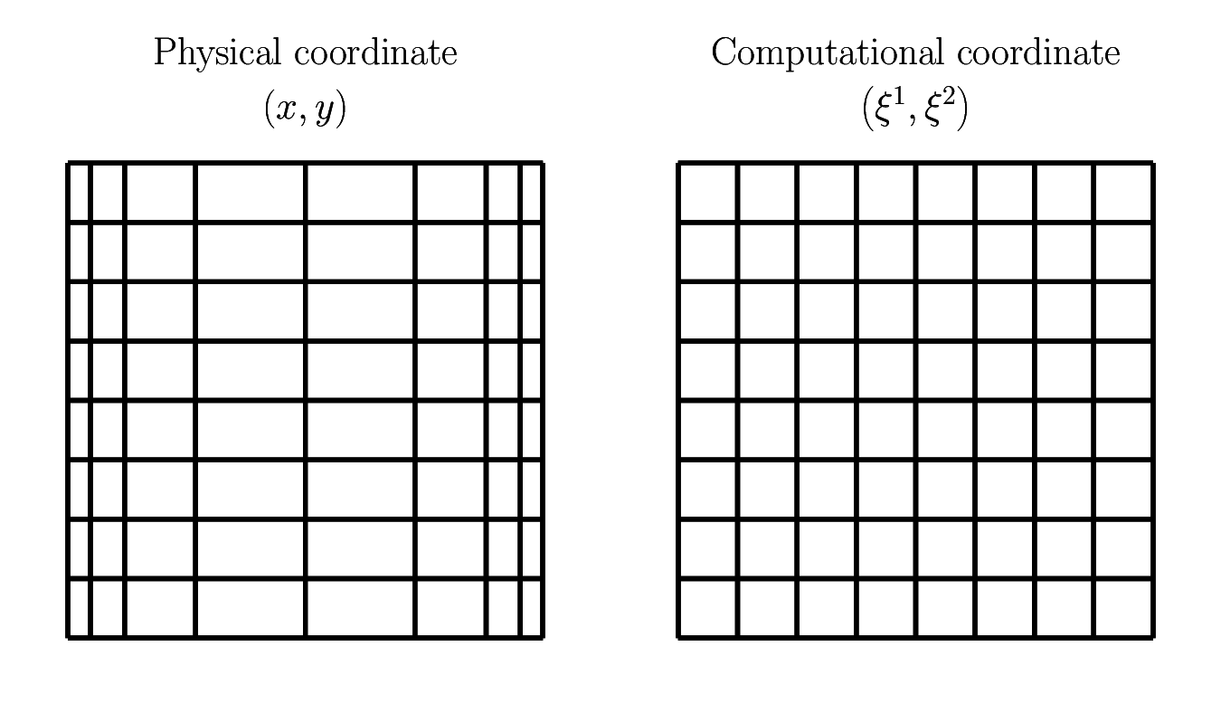
As explained in the domain setup, non-uniform grid spacings are adopted in the wall-normal direction to resolve boundary layers. This makes interpolations of quantities ambiguous, as linear interpolations, arithmetic averages, and volumetric averages all yield different results. As Ham et al., J. Comput. Phys. (177), 2002 pointed out, to obtain discrete advective terms that are energy-conserving, we need to utilize the volumetric averages to average some quantities, while arithmetic averages should be used for others, which is cumbersome and error-prone to implement. To mitigate this issue, we perform a coordinate transform from the original coordinate (physical coordinate) to a new coordinate (computational coordinate):

Since the cell-face distances are always unity in the new coordinate system, arithmetic averages suffice for all interpolations. This is a versatile approach and is applicable to the other coordinate systems as well.

Note, however, that the new coordinate system has different basis vectors compared to the original system. The wall-normal basis vectors in the physical coordinate system are \(\basis{1}\) with a unique length everywhere, while \(\gbasis{1}\) varies in size. We need to take this kind of stretching of the coordinates into account. To this end, we write down the governing equations in a more general way, incorporating the spatial changes in the basis vectors (strong conservation form for rectilinear coordinates), giving the following relations:

\[\frac{1}{J} \pder{}{\gcs{j}} \left( J \gvel{j} \right) = 0,\]

\[\gbasis{i} \left[ \pder{\gvel{i}}{t} + \frac{\gvel{j}}{\sfact{i}} \pder{}{\gcs{j}} \left( \sfact{i} \gvel{i} \right) + \frac{1}{\sfact{i}} \frac{1}{\sfact{i}} \pder{p}{\gcs{i}} - \frac{\sqrt{Pr}}{\sqrt{Ra}} \frac{1}{\sfact{i}} \frac{1}{J} \pder{}{\gcs{j}} \left\{ \frac{J}{\sfact{j}} \frac{1}{\sfact{j}} \pder{}{\gcs{j}} \left( \sfact{i} \gvel{i} \right) \right\} - \frac{T}{\sfact{1}} \delta_{i1} \right] = 0_i,\]

\[\pder{T}{t} + \gvel{j} \pder{T}{\gcs{j}} - \frac{1}{\sqrt{Pr} \sqrt{Ra}} \frac{1}{J} \pder{}{\gcs{j}} \left( \frac{J}{\sfact{j}} \frac{1}{\sfact{j}} \pder{T}{\gcs{j}} \right) = 0.\]

\(\gvel{i}\) are the contra-variant components of the velocity vector with co-variant basis vectors, i.e.,

\[\vec{u} \equiv \basis{i} u_i \equiv \gbasis{i} \gvel{i}.\]

The basis vectors and the components of the two coordinate systems are related by

\[ \begin{align}\begin{aligned}\basis{i} & = \pder{\gcs{j}}{x_i} \gbasis{j},\\u_i & = \pder{x_i}{\gcs{j}} \gvel{j},\end{aligned}\end{align} \]

or for rectilinear coordinates simply

\[ \begin{align}\begin{aligned}\basis{i} & = \pder{\gcs{i}}{x_i} \gbasis{i} \equiv \frac{1}{\sfact{i}} \gbasis{i} \,\, (\text{no summation rule over}\,i),\\u_i & = \pder{x_i}{\gcs{i}} \gvel{i} \equiv \sfact{i} \gvel{i} \,\, (\text{no summation rule over}\,i),\end{aligned}\end{align} \]

where \(\sfact{i}\) is the scale factor. Since we design the computational coordinate systems such that the grid sizes are unitary, the scale factors are given by the grid sizes in the physical coordinates:

\[ \begin{align}\begin{aligned}\sfact{1} & \equiv \Delta x,\\\sfact{2} & \equiv \Delta y,\\\sfact{3} & \equiv \Delta z,\end{aligned}\end{align} \]

which are implemented in the code as follows.

Note that, since the wall-normal grid sizes may differ, the wall-normal scale factors \(\sfact{1}\) are stored at every wall-normal cell face and center. At the faces, we calculate them using the cell-center distance

\[\vat{\sfact{1}}{\cmidx{i}} = \vat{x}{i} - \vat{x}{i-1}:\]

src/domain.c

static double * allocate_and_init_hxxf (
    const int isize,
    const double * xc
) {
  double * hxxf = memory_calloc(isize + 1, sizeof(double));
  for (int i = 1; i <= isize + 1; i++) {
    HXXF(i  ) = XC(i  ) - XC(i-1);
  }
  return hxxf;
}

At the centers, we calculate them using the cell-face distance

\[\vat{\sfact{1}}{\ccidx{i}} = \vat{x}{\cpidx{1}} - \vat{x}{\cmidx{1}}:\]

src/domain.c

static double * allocate_and_init_hxxc (
    const int isize,
    const double * xf
) {
  double * hxxc = memory_calloc(isize, sizeof(double));
  for (int i = 1; i <= isize; i++) {
    HXXC(i  ) = XF(i+1) - XF(i  );
  }
  return hxxc;
}

The scale factors in the other directions (\(\sfact{2}, \sfact{3}\)) are constant across the whole domain as we fix the grid sizes equidistant:

src/domain.c

*hy = lengths[1] / glsizes[1];

src/domain.c

*hz = lengths[2] / glsizes[2];

Note that, by definition, the Jacobian determinant is given by

\[J = \Pi_i \sfact{i},\]

which are implemented in the code as follows. Note that they are also defined at the wall-normal cell faces and centers:

src/domain.c

static double * allocate_and_init_jdxf (
    const int isize,
    const double * hxxf,
#if NDIMS == 2
    const double hy
#else
    const double hy,
    const double hz
#endif
) {
  double * jdxf = memory_calloc(isize + 1, sizeof(double));
  for (int i = 1; i <= isize + 1; i++) {
#if NDIMS == 2
    JDXF(i  ) = HXXF(i  ) * hy;
#else
    JDXF(i  ) = HXXF(i  ) * hy * hz;
#endif
  }
  return jdxf;
}

src/domain.c

static double * allocate_and_init_jdxc (
    const int isize,
    const double * hxxc,
#if NDIMS == 2
    const double hy
#else
    const double hy,
    const double hz
#endif
) {
  double * jdxc = memory_calloc(isize, sizeof(double));
  for (int i = 1; i <= isize; i++) {
#if NDIMS == 2
    JDXC(i  ) = HXXC(i  ) * hy;
#else
    JDXC(i  ) = HXXC(i  ) * hy * hz;
#endif
  }
  return jdxc;
}

Finally, since we usually discuss everything on the physical coordinate systems rather than on the computational coordinate systems, it is convenient to keep the velocity vector descriptions using \(\vel{i}\) rather than \(\gvel{i}\), giving

\[\frac{1}{J} \pder{}{\gcs{j}} \left( \frac{J}{\sfact{j}} \vel{j} \right) = 0,\]

\[\basis{i} \left\{ \pder{\vel{i}}{t} + \frac{\vel{j}}{\sfact{j}} \pder{\vel{i}}{\gcs{j}} + \frac{1}{\sfact{i}} \pder{p}{\gcs{i}} - \frac{\sqrt{Pr}}{\sqrt{Ra}} \frac{1}{J} \pder{}{\gcs{j}} \left( \frac{J}{\sfact{j}} \frac{1}{\sfact{j}} \pder{\vel{i}}{\gcs{j}} \right) - T \delta_{i1} \right\} = 0_i,\]

\[\pder{T}{t} + \frac{\vel{j}}{\sfact{j}} \pder{T}{\gcs{j}} - \frac{1}{\sqrt{Pr} \sqrt{Ra}} \frac{1}{J} \pder{}{\gcs{j}} \left( \frac{J}{\sfact{j}} \frac{1}{\sfact{j}} \pder{T}{\gcs{j}} \right) = 0,\]

as a set of conclusive equations.

See also

For detailed derivation of the mentioned relations, visit this page.